Since Microsoft Excel is such a popular and heavily-used program in the world today, it’s important to understand the basics of the program no matter what you do in life.
Sometimes when working with Excel, you input phrases or numbers that are longer than the unedited cell size, which ends up looking confusing to some beginners. The text or numbers could spill over into the next cell and this could make it hard to work on your spreadsheet.
If this happens to you often and you are not sure of how to edit your cells in order to facilitate large texts or figures, here are three easy tips for getting this aspect of using Excel under your belt.
1. AutoFitting the rows and columns
This is a more advanced way to deal with this issue, but it’s probably the best and fastest way to do it in the long run so that you don’t have to continually edit your cells. Once you input these parameters, they will be enforced on your entire spreadsheet.
Select the spreadsheet or the part of the spreadsheet that you want to format.
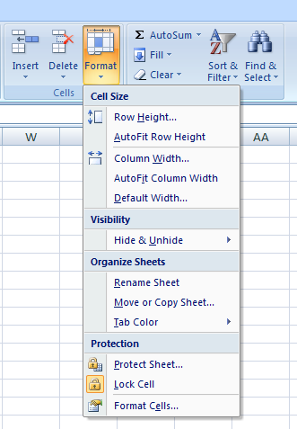
Click “Format” on the main menu, and then click on “AutoFit Row Height” or “AutoFit Column Width,” depending on what you want.
2. Shrink to fit
Another simple way to make your text fit is to shrink the text. However, keep in mind that this will leave you with different sized text all over your spreadsheet, which won’t look very uniform.
Click again on “Format,” and then click on “Format Cells…”
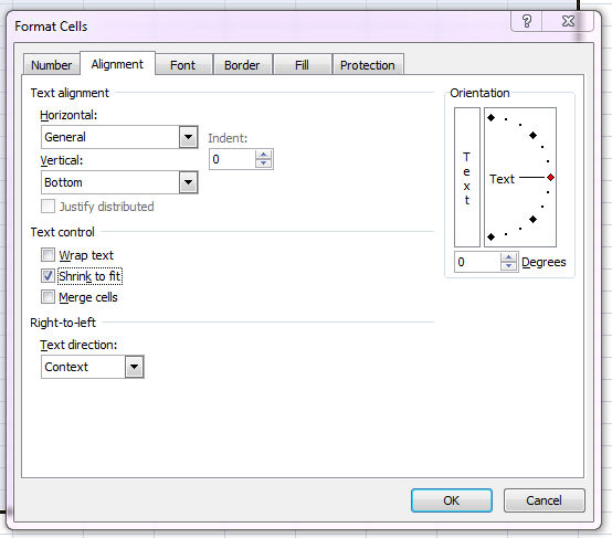
Go to the “Alignment” tab.
Click on “Shrink to fit” and then click “OK.”
3. Do it manually
You can also change the height and width of your rows and columns manually.
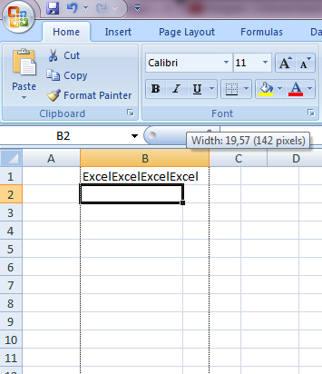
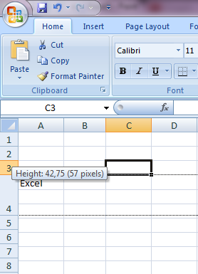
Put the mouse on the end of the row or column so that the cursor changes to one that shows arrows on both sides. Click and hold the mouse to drag the row or column line to your desired size.


